


Introduction
You can analyze Cajori Two data in two ways.
1. The Online approach – what this file is aimed at. You get to this capability by clicking the website button entitled Online Data Analysis Tool. This is excellent for browsing.
2. The Download-for-Excel approach. You need to download some files (there is a button for this which you get to by clicking Download for Excel Analysis). You will need Excel installed to make use of the downloaded files. If you are beyond browsing and want to make a permanent record of some data, you might find it worthwhile learning how this works.
This file has 4 sections, of which the first 2 are useful knowledge for whichever method you choose. The last two sections specifically concern the Online approach, including some examples explained at the “click here” level. For details of the Download-for-Excel approach, see the file DownloadForExcelPerspectiveAndExamples.docx in the following subfolder of the downloaded folder: CajoriTwo_4.0\DataAnalysis
The technically inclined might find it interesting to know that the Online approach operates by having the data base software MySQL respond to your requests. No knowledge of MySQL is needed by the user. For the Download-for-Excel approach, your requests are satisfied by the Excel-based Data Analysis Software1 written in the VBA programming language. This VBA language is built in to every Windows version of Excel and many Macintosh versions as well. You will need to have Excel installed to use the Download-for-Excel approach.
Section 1. General Remarks I: Summary and Comparison of Online Analysis and Analysis Via the Download-for-Excel approach
Section 2. General Remarks II: Avoiding Unfortunate Interpretations
Section 3. Directed Online Investigations – “Click here” Examples
Section 4: Decision Tree for Selecting an Online Summing Option
Section 1. General Remarks I: Summary and Comparison of Online Analysis and Analysis Via the Download-for-Excel Approach
The capabilities of the Online approach and the Download-for-Excel approach are mostly the same, but there are some differences:
Selecting years. You can leave some years out of time-series tables calculated for you by the Online approach, but in the Download-for-Excel approach each year is reported and you have to ignore the ones you don’t want.
Selecting courses. In in the Download-for-Excel approach you take all of a course category or none. In The Online approach you can leave out any courses you like from a category.
Custom category. You can create a custom category, with courses chosen from other categories in in the Download-for-Excel approach. This is not possible in the Online approach.
In the Online approach, the numbers you want come up in a table on the screen. If you want a permanent record of them, you must download the table to your own machine2. It will appear in the form of an Excel workbook containing the table. Unfortunately, there is no labeling or titling of the table. You will have to make notes about the numbers you have generated (what the numbers mean, what departments participated in the analysis, what course categories, etc.) and immediately annotate your download so that its meaning does not get lost. These labelings are provided for you automatically by the Download-for-Excel approach. There are also some filing aspects concerning the downloaded Excel workbook under the Online approach. What should you name the workbook? In what folder should you place it? If there were only 2 or 3 tables these issues would matter little, but there are 49. You may like the “do-it-yourself” control the Online approach offers, or you may prefer to have it all done for you as is the case with the Download-for-Excel approach.
Instructions for creating tables using the Download-for-Excel approach can be found in the file AnalysisAfterDownloadPerspectiveAndExamples.docx within the CajoriTwo_4.0\DataAnalysis subfolder of the downloaded folder.
Section 2. General Remarks II: Subsets to Avoid Unfortunate Interpretations
There are 25 departments in our database. You don’t need to use them all in a run of the data and we suggest that most of the time you won’t want them all. Here are some reasons:
Some departments do not show a calculus course in 1905 (0 presences and instances in the corresponding cell.) Can it be that calculus was not universal early in the century? Actually, it was. But some of our departments did not exist in 1905 (e.g., the Johns Hopkins Dep’t of Applied Mathematics and Statistics did not come into being, as a sister department of the pre-existing department of mathematics, till 1975.) In some cases, the institution housing one of our 25 departments did not exist till later. (Reed College did not exist in 1905.) In another case, the institution and department did exist but the archivist could not find any catalogs till 1936 (Morgan State University.) In such cases, you can ignore some years to avoid the spurious zeros. Alternatively you can ask for data involving a subset of the 25 departments.
Another reason one might want to run the data for a subset of the departments is that one wants to deal just with a special group of institutions, e.g., larger institutions.
Depending on your degree of fussiness, you might wish to ignore the U. S. Military Academy at West Point, because this important and interesting institution did not, for some of its history, have a curricular structure organized around courses in the conventional way. For example, early in the century you will find that second year mathematics included Calculus, Descriptive Geometry and Least Squares. But how much time each of these three subjects was allotted is not recorded. West Point quite commonly would switch from one subject to a mostly unrelated one in the middle of a semester, and perhaps devote just a short time to it. Thus, when we report a descriptive geometry “course” for West Point, this is actually a fiction, because it is a topic within a year of mathematics.
Finally, in the matter of leaving departments out of the analysis, it is essential to think about the role of “combination departments” (“combos” for short). A combination department is a fictitious department created by us for those campuses where there are multiple mathematics departments (“sister departments”). It represents the totality of mathematics available to an undergraduate at that campus. If, for example, one includes the combination of all mathematics departments at the U. of Texas at Austin in a summation, one probably would not want to include any of the individual actual departments at that campus. The reason is that any course at an individual department, say Solid Geometry in the applied mathematics department of 1925-26, will also be present in the combination department. Thus, this course will be counted twice in any sums taken over the departments and combos you have included in your analysis.
Categories can also be omitted form the analysis. Computer science3 is an example of a category of courses you may wish to ignore. (Since some time in the 1980’s, NSF has not regarded Computer Science as being included in the category it calls Mathematical Sciences.) Alternatively, you might be uninterested in the two most elementary categories if you are interested mostly in what courses mathematics majors study in the latter part of the century. As with unwanted departments or combinations, there are some tables where you can simply disregard what is reported about categories you want to ignore. However, in some tables involving data summed over categories, the presence of the unwanted categories may skew the data in a way that can not be corrected by any form of looking away.
Section 3. Directed Online Investigations – “Click here” Examples
Here are some examples of how one might use the available tables to study questions of interest. Our illustrations will use the on-line data analysis tool based on MySQL, but the same questions could be pursued through the Download-for-Excel approach where one runs the Excel-based Data Analysis Software on the downloaded files. (To find the Excel-based Data Analysis Software, and some explanations concerning it, click the button entitled Download for Excel Analysis and download the CajoriTwo_4.0 folder available after your click.)
The Size of the Mathematics Teaching Enterprise
The 20th century was the century of “ever more” in most areas of American life: population, affluence, educational opportunity, pollution, etc. Was this true of mathematics teaching also? One way to document this is to take some particular school and see how many mathematics courses it had at the different time points of our survey: 1905, 1915, . . . , 2005.
Start from the Home page and do these clicks:
• Online Data Analysis Tool > Begin Your Search
• In the center of the screen, above the “Search” button, click “time series”. This means you want numbers for a series of years.
• In the left hand column select a campus, say Johns Hopkins U.’s Mathematics Department4.
• Next, click the box next to “Decades” to assert that you want all decades. (You could instead pick decades individually by leaving the previously mentioned box alone and clicking the individual decade boxes.)
• Next check the box next to “Categories/Courses” if you want all courses in all categories. (You could, instead, leave that box unclicked and then click individual categories. For example, maybe you want to see how the most elementary category of course grew or shrank over the years. If you want to be even more specific, you could click a plus sign next to a category in order to select particular courses in the category.)
• Now click “Search”.
Examine the box above the display of courses and years. You will see “course presences” clicked. A “1” for course 17 in category 1 in 1905 means that one or more courses in Comprehensive Preparation For Calculus5 were taught. We can’t tell from this exactly how many variants or instances of this course there were. If you want to count instances, you have to click the button for instances, and then you would find that there were 2 (maybe it was a 2-semester course and the two semesters were the two instances, or maybe there was a 1-semester version for science students and another semester version for everyone else, or maybe one was an honors version of the other, or maybe one was an experimental version. )
The main part of the screen is a table of course presences (or maybe instances), year-by-year. This allows us to study individual courses. But the question we started with had to do with the totality of courses, which we might interpret as a totality of presences. To get this we need to select a summing option in the right hand side of the box under the colored search button. Click option #6 6. Now the large table has been replaced by a single line of data from which we can see that course presences have steadily increased during the 20th century.
This can be done for a selection of departments. For example, if we select both Hopkins departments but go through all other steps in the same way, we can get the year by year totality of math courses at the union of both mathematics departments at Johns Hopkins. (Instead, you could just use the “combo” department for Hopkins.) One could, in this way get the sum of all departments in the sample.What are the most popular courses?
Are there courses that most departments of interest to you have in most years of their existence? We would call these popular courses. Surely 1st semester mainstream Calculus is such a course. Where does College Algebra rank? Introductory Statistics? Discrete Mathematics?
By the way, before we describe the clicks and results in this area, you might want to note that there are courses, like Quaternions that never showed up in any department of our survey even though these courses are in our inventory. Quaternions had some popularity in the 19th century, and that is why it is one our list. We made our list, in advance of looking at the data, and tried to overshoot the mark on what we might find.
Now, to pursue popularity:
• From the Home page, click on Online Data Analysis.
• Then click on Begin Your Search.
• There are three radio buttons with a lot of space to the right and left. Click the one entitled “View by course popularity”. But before you click the Search button you will have to choose the departments for which you want data. Suppose you choose the two Hopkins departments, the 3 Stanford departments and Morgan State’s mathematics department. A brief side remark: the italicized word combination next to Hopkins, and also Stanford, is explained in a “help popup” which you can read if you click on the word.
• Now let’s select all decades (just one click, in the box next to “Decades”) and all courses in all categories (1 click).
• Now click the Search button.
The numbers you see are sums over all chosen decades and all departments chosen.
The history of individual courses.
Perhaps you are interested in when individual courses were created or terminated and how individual schools differed in this respect. In this case, after clicking “Online Data Analysis Tool” and “begin your search”
• Select the departments of interest
• Select all decades
• Select just the courses you are interested in
• Select “View as a time series table”
• Click Search
• Choose “Use course presences” or “Use course instances”, as you think best
• Choose summing option 1.
A slightly different way of looking at this issue is to use the Download-for-Excel approach instead of the Online approach. After running the Excel-based Data Analysis Software in the Download-for-Excel approach, consult the first four columns of Table 2 or Table. This presentation of course histories is not available in the Online approach described in this file, although you can construct it for yourself from the information presented in response to the clicks just now mentioned.
Sortable Lists
The capability described here is a capability quite standard in dealing with databases – it came “for free”. Whether it is helpful in this project is unclear, but here is how it might work.
• If you click Online Data Analysis Tool > Begin Your Search
• and then you click the radio button “Sortable List” what you will find is a list with the following contents:
For every course you have selected,
For every department you have selected,
For every year you have selected:
an indication whether a course of that type is present (0 or 1 in the presences column), and how many instances (variants) there were, in the instances column.
Let’s try this out to investigate how Stanford as a whole (combining all departments) compares in 1905 to 2005 in the course category entitled Analysis Following Basic Calculus. Begin by clicking as follows:
• Online Data Analysis > Begin Your Search.
• Now select Stanford U. (combination),
• select the decades containing years 1905 and 2005, and
• select the Analysis Following Basic Calculus category.
• Make sure the “View as a sortable list” radio button is clicked.
• Now click “Search”.
You will see a sprinkling of non-zero integers. Even without doing any sorting, you might draw some conclusions. But let’s see if sorting adds anything.
Let’s say we want to sort in the following sequence: first by year (so we’ll keep all the 1905 results together and the 2005 ones together); then by instances. How can we do this? First notice that “Year” header box at the top of the table will be filled in in blue. This shows the variable on which some sorting has already been done. To say that, we want secondary sorting by instances, within that sorting by year, hold the shift key down and click the “Instances” column heads. What happens now is that, within all the 1905 results, they will be sorted by instances, and within the 2005 results all will be sorted by instances. It is a separate sort for each year. You can have as many sorts nested within one another as you like. But if you don’t hold the shift key down and click a column you will be starting up a whole new set of sorts – previous choices of how to sort are wiped out.
At this point we can see the non-zero instances together. For 2005 there are 6 of them and in 1905 only 3. Also note that there are some newcomers in 2005: Numerical Analysis, Complex Analysis and Introduction to Functional Analysis/Linear Operators.
A few more thoughts about the technicalities of sorting:• If you want results in ascending order click the arrow in the column heading.
• Whenever you select more than one column, the question arises about what order the various columns are used to sort. It goes according to the order in which you clicked the columns. For example if you have chosen Years first then Campus/Department, all 1905 entries are consecutively together. Within the grouping of 1905 entries they are sorted by department. If you wanted all Johns Hopkins Applied Mathematics and Statistics courses to be consecutively together, and within the Johns Hopkins Applied Mathematics courses you next wanted the courses sorted by year, then click Campus/Department first, then click Year.
Material Under Construction
The last sheet, Births&Deaths in the file CourseHistoriesAllDeptOrCombos.xlsx (you will find this in the sample output and most other output you generate ) contains material that we do notconsider fully developed in regard to verified accuracy or wisdom. It is generated by the codein the module ForCourseHistoriesM which is in the file CountsIndivDeptsOrCombos.xlsx.
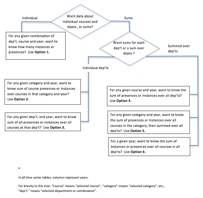
Section 4: Decision Tree for Selecting an Online Summing Option Option
1We wrote the VBA code in the Windows version of VBA. This is said to almost 100% identical to the Macintosh version, but we have not tried our code on a Mac, so we recommend using Windows if possible.
2For the analyst who wants a permanent record of his or her explorations, the two approaches might best be called “download now” and “download later” as both require downloading. Both also require Excel, but only the very slightest knowledge of how to use Excel.
3We deal only with computer-related courses that have a “mathematics designation”. For example we ignore “CS150 Algorithms”, but if it were “M150 Algorithms” we include it.
4If you choose the Applied Mathematics and Statistics Department, you would have to be aware that this department did not exist for the early part of the 20th century. This can be seen in the many zeros when you examine this department.
5If you want to know what we mean by these course titles, click the button Download for Excel Analysis on the website. Next download the folder CajoriTwo_4.0 and look in CajoriTwo_4.0> AbbreviatedCatalogData>HowTheAbbreviatedDataWasProduced>GeneralMethodology>ClusteredInventory.docx.
6By hovering, with the mouse, over the title of the option you will find a longer description of that summing option along with the number of the table when it is produced by the Download-for-Excel approach and the Excel-based Data Analysis Software. By clicking on Help you can find even more information.